Executing Projects

This section describes how executing a project works and what resources are passed between project items at execution time. The buttons used to control executions are located in the Toolbar’s Execute -section. Execution happens by either pressing the Project button () to execute the whole project, or by pressing the Selection button () to only execute selected items. Next to these buttons is the Stop button (), which can be used to stop an ongoing execution. A project consists of project items and connections (yellow arrows) that are visualized on the Design View. You use the project items and the connections to build a Directed Acyclic Graph (DAG), with the project items as nodes and the connections as edges. A DAG is traversed using the breadth-first-search algorithm.

Rules of DAGs:

1. A single project item with no connections is a DAG.

2. All project items that are connected, are considered as a single DAG (no matter, which direction the arrows go). If there is a path between two items, they are considered as belonging to the same DAG.

3. Loops are not allowed (this is what acyclic means).

You can connect the nodes in the Design View how ever you want but you cannot execute the resulting DAGs if they break the rules above. Here is an example project with three DAGs.

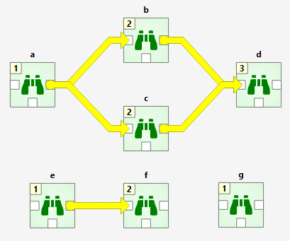
• DAG 1: items: a, b, c, d. connections: a-b, a-c, b-d, c-d

• DAG 2: items: e, f. connections: e-f

• DAG 3: items: g. connections: None

The numbers on the upper left corners of the icons show the item’s execution ranks which roughly tell the order of execution within a DAG. Execution order of DAG 1 is a->b->c->d or a->c->b->d because b and c are siblings which is also indicated by their equal execution rank. DAG 2 execution order is e->f and DAG 3 is just g. All three DAGs are executed in a row though which DAG gets executed first is undefined. Therefore all DAGs have their execution ranks starting from 1.

We use the words predecessor and successor to refer to project items that are upstream or downstream from a project item. Direct predecessor is a project item that is the immediate predecessor while Direct Successor is a project item that is the immediate successor. For example, in the DAG 1 presented before, the successors of a are project items b, c and d. The direct successor of b is d. The predecessor of b is a, which is also its direct predecessor.

After you press the button, you can follow the progress and the current executed item in the Event Log. Design view also animates the execution.

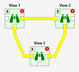
Items in a DAG that breaks the rules above are marked by X as their rank. Such DAGs are skipped during execution. The image below shows such a DAG where the items form a loop.

You can also execute only the selected parts of a project by multi-selecting the items you want to execute and pressing the button in the tool bar. For example, to execute only items b, d and f, select the items in Design View or in the project item list in Project dock widget and then press the button.

Tip

You can select multiple project items by holding the Ctrl key down and clicking on desired items or by drawing a rectangle on the Design view.

Example DAG

When you have created at least one Tool specification, you can execute a Tool as part of the DAG. The Tool specification defines the process that is executed by the Tool project item. As an example, below we have two project items; Data Files Data Connection and Julia model Tool connected to each other.

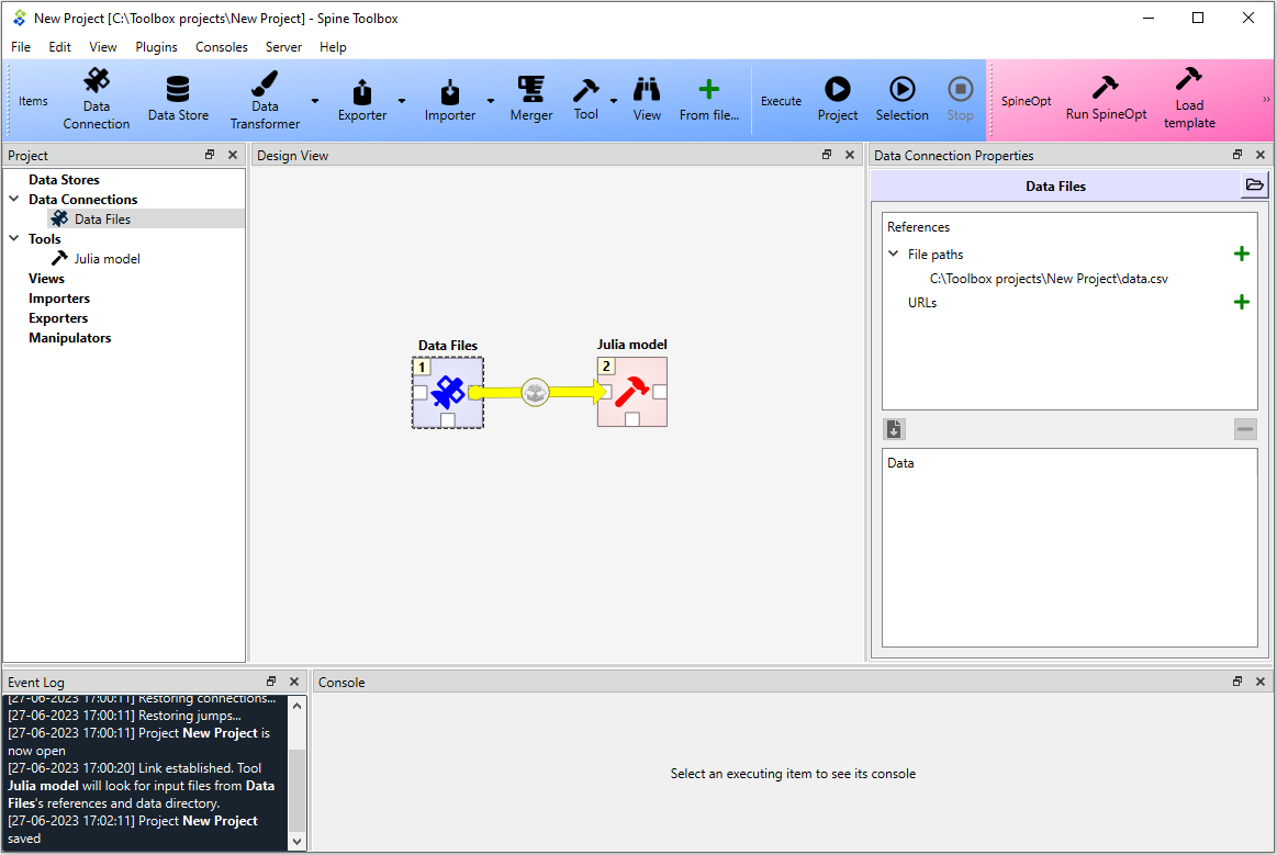
In ths example, Data Files has a single file reference data.csv. Data Connections make their files visible to direct successors and thus the connection between Data Files and Julia model provides data.csv to the latter.

Selecting the Julia model shows its properties in the Properties dock widget.

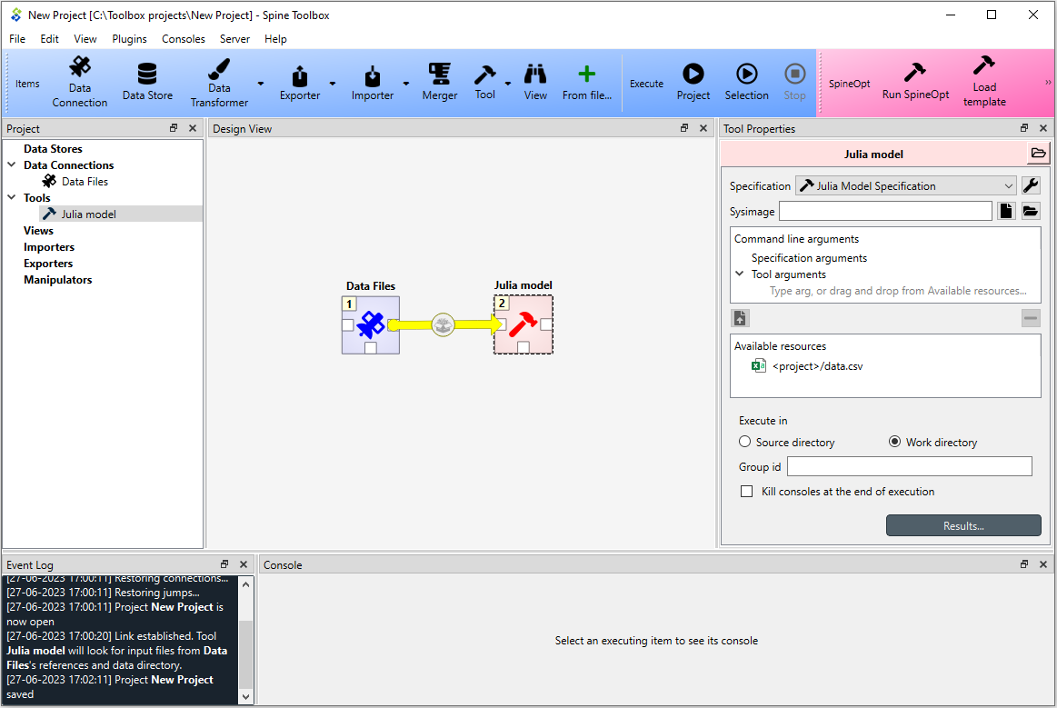
In the top of the Tool Properties, there is Specification drop-down menu. From this drop-down menu, you can select the Tool specification for this particular Tool item. The Julia Model Specification tool specification has been selected for Julia model. Below the drop-down menu, you can choose a precompiled sysimage and edit Tool’s command line arguments. Note that the command line argument editor already ‘sees’ the data.csv file provided by Data Files. The Execute in radio buttons control, whether this Tool is first copied to a work directory and executed there, or if the execution should happen in the source directory where the main program file is located. In Group id, an execution group identifier can be given. Below that, there is a checkbox with the choice to kill consoles after execution. Results… button opens the Tool’s result archive directory in system’s file browser (all Tools have their own result directory).

When you click on the button, the execution starts from the Data Files Data Connection as indicated by the execution rank numbers. When executed, Data Connection items advertise their files and references to project items that are their direct successors. In this particular example, data.csv contained in Data Files is also a required input file in Julia model Specification. When it is the Julia model tool’s turn to be executed, it checks if it finds the data.csv from its direct predecessor items that have already been executed. Once the input file has been found the Tool starts processing the main program file script.jl. Note that if the connection would be the other way around (from Julia Model to Data Files) execution would start from the Julia model and it would fail because it cannot find the required data.csv. The same thing happens if there is no connection between the two project items. In this case the project items would be in separate DAGs.

Since the Tool specification type was set as Julia and the main program is a Julia script, Spine Toolbox starts the execution in the Julia Console (if you have selected this in the application Settings, See Settings section).