Case Study A5 tutorial
Welcome to Spine Toolbox’s Case Study A5 tutorial. Case Study A5 is one of the Spine Project case studies designed to verify Toolbox and Model capabilities. To this end, it reproduces an already existing study about hydropower on the Skellefte river, which models one week of operation of the fifteen power stations along the river.
This tutorial provides a step-by-step guide to run Case Study A5 on Spine Toolbox and is organized as follows:
Introduction
Model assumptions
For each power station in the river, the following information is known:
The capacity, or maximum electricity output. This datum also provides the maximum water discharge as per the efficiency curve (see next point).
The efficiency curve, or conversion rate from water to electricity. In this study, a piece-wise linear efficiency with two segments is assumed. Moreover, this curve is monotonically decreasing, i.e., the efficiency in the first segment is strictly greater than the efficiency in the second segment.
The maximum magazine level, or amount of water that can be stored in the reservoir.
The magazine level at the beginning of the simulation period, and at the end.
The minimum amount of water that the plant needs to discharge at every hour. This is usually zero (except for one of the plants).
The minimum amount of water that needs to be spilled at every hour. Spilled water does not go through the turbine and thus does not serve to produce electricity; it just helps keeping the magazine level at bay.
The downstream plant, or next plant in the river course.
The time that it takes for the water to reach the downstream plant. This time can be different depending on whether the water is discharged (goes through the turbine) or spilled.
The local inflow, or amount of water that naturally enters the reservoir at every hour. In this study, it is assumed constant over the entire simulation period.
The hourly average water discharge. It is assumed that before the beginning of the simulation, this amount of water has constantly been discharged at every hour.
The system is operated so as to maximize total profit over the week, while respecting capacity constraints, maximum magazine level constrains, and so on. Hourly profit per plant is simply computed as the product of the electricity price and the production, minus a penalty for changes on the water discharge in two consecutive hours. This penalty is computed as the product of a constant penalty factor, common to all plants, and the absolute value of the difference in discharge with respect to the previous hour.
Modelling choices
The model of the electric system is fairly simple, only two elements are needed:
A common electricity node.
A load unit that takes electricity from that node.
On the contrary, the model of the river system is more detailed. Each power station in the river is modelled using the following elements:
An upper water node, located at the entrance of the station.
A lower water node, located at the exit of the station.
A power plant unit, that discharges water from the upper node into the lower node, and feeds electricity produced in the process to the common electricity node.
A spillway connection, that takes spilled water from the upper node and releases it to the downstream upper node.
A discharge connection, that takes water from the lower node and releases it to the downstream upper node.
Below is a schematic of the model. For clarity, only the Rebnis station is presented in full detail:

Guide
Installing requirements
Note
This tutorial is written for latest Spine Toolbox and SpineOpt development versions.
Follow the instructions here to install Spine Toolbox and SpineOpt in your system.
Creating a new project
Each Spine Toolbox project resides in its own directory, where the user can store data, programming scripts and other necessary material. The Toolbox application also creates its own special subdirectory .spinetoolbox, for project settings, etc.
To create a new project, select File -> New project… from Spine Toolbox main menu. Browse to a location where you want to create the project and create a new folder for it, called e.g. ‘Case Study A5’, and then click Open.
Configuring SpineOpt
To use SpineOpt in your project, you need to create a Tool specification for it. Click on the small arrow next to the Tool icon
 (in the Main section of the tool bar),
and press New…
The Tool specification editor will popup:
(in the Main section of the tool bar),
and press New…
The Tool specification editor will popup: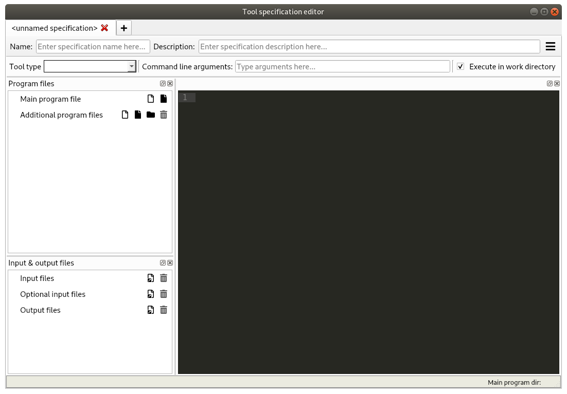
Type ‘SpineOpt’ as the name of the specification and select ‘Julia’ as the type. Unselect Execute in work directory.
Press
 next to Main program file to create a new Julia file.
Enter a file name, e.g. ‘run_spineopt.jl’, and click Save.
next to Main program file to create a new Julia file.
Enter a file name, e.g. ‘run_spineopt.jl’, and click Save.Back in the Tool specification editor form, select the file you just created under Main program file. Then, enter the following text in the text editor to the right:
using SpineOpt

run_spineopt(ARGS...)
At this point, the form should be looking similar to this:

Press Ctrl+S to save everything, then close the Tool specification editor.
Setting up project
Drag the Data Store icon
 from the tool bar and drop it into the
Design View. This will open the Add Data Store dialog.
Type ‘input’ as the Data Store name and click Ok.
from the tool bar and drop it into the
Design View. This will open the Add Data Store dialog.
Type ‘input’ as the Data Store name and click Ok.Repeat the above procedure to create a Data Store called ‘output’.
Create a database for the ‘input‘ Data Store:
Select the input Data Store item in the Design View to show the Data Store Properties (on the right side of the window, usually).
In Data Store Properties, select the sqlite dialect at the top, and hit New Spine db.
Repeat the above procedure to create a database for the ‘output’ Data Store.
Click on the small arrow next to the Tool icon
and drag the ‘SpineOpt’
item from the drop-down menu into the Design View.
This will open the Add Tool dialog. Type ‘SpineOpt’ as the Tool name and click Ok.Note
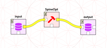
Each item in the Design view is equipped with three connectors (the small squares at the item boundaries).
Click on one of ‘input’ connectors and then on one of ‘SpineOpt’ connectors. This will create a connection from the former to the latter.
Repeat the procedure to create a connection from SpineOpt to output. It should look something like this:
Setup the arguments for the SpineOpt Tool:
Select the SpineOpt Tool to show the Tool Properties (on the right side of the window, usually). You should see two elements listed under Available resources,
{db_url@input}and{db_url@output}.Drag the first resource,
{db_url@input}, and drop it in Command line arguments, just as shown in the image below.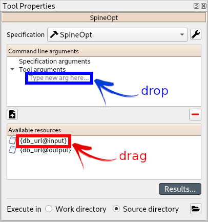
Drag the second resource,
{db_url@output}, and drop it right below the previous one. The panel should be now looking like this: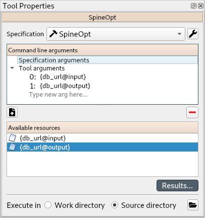
Double-check that the order of the arguments is correct: first,
{db_url@input}, and second,{db_url@output}. (You can drag and drop to reorganize them if needed.)
From the main menu, select File -> Save project.
Entering input data
Importing the SpineOpt database template
Download the SpineOpt database template (right click on the link, then select Save link as…)
Select the input Data Store item in the Design View.
Go to Data Store Properties and hit Open editor. This will open the newly created database in the Spine DB editor, looking similar to this:

Note
The Spine DB editor is a dedicated interface within Spine Toolbox for visualizing and managing Spine databases.
Press Alt + F to display the main menu, select File -> Import…, and then select the template file you previously downloaded. The contents of that file will be imported into the current database, and you should then see classes like ‘commodity’, ‘connection’ and ‘model’ under the root node in the Object tree (on the left).
From the main menu, select Session -> Commit. Enter ‘Import SpineOpt template’ as message in the popup dialog, and click Commit.
Note
The SpineOpt template contains the fundamental object and relationship classes, as well as parameter definitions, that SpineOpt recognizes and expects. You can think of it as the generic structure of the model, as opposed to the specific data for a particular instance. In the remainder of this section, we will add that specific data for the Skellefte river.
Creating objects
Add power plants to the model. Create objects of class
unitas follows:Select the list of plant names from the text-box below and copy it to the clipboard (Ctrl+C):
Rebnis_pwr_plant
Sadva_pwr_plant
Bergnäs_pwr_plant
Slagnäs_pwr_plant
Bastusel_pwr_plant
Grytfors_pwr_plant
Gallejaur_pwr_plant
Vargfors_pwr_plant
Rengård_pwr_plant
Båtfors_pwr_plant
Finnfors_pwr_plant
Granfors_pwr_plant
Krångfors_pwr_plant
Selsfors_pwr_plant
Kvistforsen_pwr_plant
Go to Object tree (on the top left of the window, usually), right-click on
unitand select Add objects from the context menu. This will open the Add objects dialog.Select the first cell under the object name column and press Ctrl+V. This will paste the list of plant names from the clipboard into that column; the object class name column will be filled automatically with ‘unit‘. The form should now be looking similar to this:
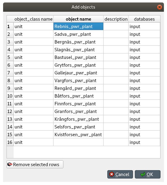
Click Ok.
Back in the Spine DB editor, under Object tree, double click on
unitto confirm that the objects are effectively there.Commit changes with the message ‘Add power plants’.
Add discharge and spillway connections. Create objects of class
connectionwith the following names:Rebnis_to_Bergnäs_disch Sadva_to_Bergnäs_disch Bergnäs_to_Slagnäs_disch Slagnäs_to_Bastusel_disch Bastusel_to_Grytfors_disch Grytfors_to_Gallejaur_disch Gallejaur_to_Vargfors_disch Vargfors_to_Rengård_disch Rengård_to_Båtfors_disch Båtfors_to_Finnfors_disch Finnfors_to_Granfors_disch Granfors_to_Krångfors_disch Krångfors_to_Selsfors_disch Selsfors_to_Kvistforsen_disch Kvistforsen_to_downstream_disch Rebnis_to_Bergnäs_spill Sadva_to_Bergnäs_spill Bergnäs_to_Slagnäs_spill Slagnäs_to_Bastusel_spill Bastusel_to_Grytfors_spill Grytfors_to_Gallejaur_spill Gallejaur_to_Vargfors_spill Vargfors_to_Rengård_spill Rengård_to_Båtfors_spill Båtfors_to_Finnfors_spill Finnfors_to_Granfors_spill Granfors_to_Krångfors_spill Krångfors_to_Selsfors_spill Selsfors_to_Kvistforsen_spill Kvistforsen_to_downstream_spill
Add water nodes. Create objects of class
nodewith the following names:Rebnis_upper Sadva_upper Bergnäs_upper Slagnäs_upper Bastusel_upper Grytfors_upper Gallejaur_upper Vargfors_upper Rengård_upper Båtfors_upper Finnfors_upper Granfors_upper Krångfors_upper Selsfors_upper Kvistforsen_upper Rebnis_lower Sadva_lower Bergnäs_lower Slagnäs_lower Bastusel_lower Grytfors_lower Gallejaur_lower Vargfors_lower Rengård_lower Båtfors_lower Finnfors_lower Granfors_lower Krångfors_lower Selsfors_lower Kvistforsen_lower
Next, create the following objects (all names in lower-case):
instanceof classmodel.waterandelectricityof classcommodity.electricity_nodeof classnode.electricity_loadof classunit.some_weekof classtemporal_block.deterministicof classstochastic_structure.realizationof classstochastic_scenario.
Finally, create the following objects to get results back from Spine Opt (again, all names in lower-case):
my_reportof classreport.unit_flow,connection_flow, andnode_stateof classoutput.
Note
To modify an object after you enter it, right click on it and select Edit… from the context menu.
Specifying object parameter values
Specify the general behaviour of our model. Enter
modelparameter values as follows:Select the model parameter value data from the text-box below and copy it to the clipboard (Ctrl+C):
model	instance	duration_unit	Base	"hour"
model	instance	model_end	Base	{"type": "date_time", "data": "2019-01-08T00:00:00"}
model	instance	model_start	Base	{"type": "date_time", "data": "2019-01-01T00:00:00"}
Go to Object parameter value (on the top-center of the window, usually). Make sure that the columns in the table are ordered as follows:
object_class_name | object_name | parameter_name | alternative_name | value | database
Select the first empty cell under
object_class_nameand press Ctrl+V. This will paste the model parameter value data from the clipboard into the table. The form should be looking like this: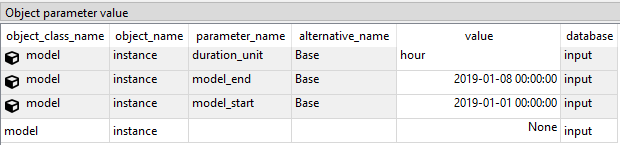
Specify the resolution of our temporal block. Repeat the same procedure with the data below:
temporal_block some_week resolution Base {"type": "duration", "data": "1h"}
Specify the behaviour of all system nodes. Repeat the same procedure with the data below, where:
demandrepresents the local inflow (negative in most cases).fix_node_staterepresents fixed reservoir levels (at the beginning and the end).has_stateindicates whether or not the node is a reservoir (true for all the upper nodes).state_coeffis the reservoir ‘efficienty’ (always 1, meaning that there aren’t any loses).node_state_capis the maximum level of the reservoirs.
node	Bastusel_upper	demand	Base	-0.2579768519
node	Bergnäs_upper	demand	Base	-22.29
node	Båtfors_upper	demand	Base	-2
node	Finnfors_upper	demand	Base	0
node	Gallejaur_upper	demand	Base	15.356962963
node	Granfors_upper	demand	Base	0
node	Grytfors_upper	demand	Base	-3.78
node	Krångfors_upper	demand	Base	0
node	Kvistforsen_upper	demand	Base	-1.3273809524
node	Rebnis_upper	demand	Base	-3.68
node	Rengård_upper	demand	Base	-10.37
node	Sadva_upper	demand	Base	-5.43
node	Selsfors_upper	demand	Base	0
node	Slagnäs_upper	demand	Base	0
node	Vargfors_upper	demand	Base	-3.5584953704
node	Bastusel_upper	fix_node_state	Base	{"type": "time_series", "data": {"2019-01-01T00:00:00": 5581.44, "2019-01-01T01:00:00": NaN, "2019-01-07T23:00:00": 5417.28}}
node	Bergnäs_upper	fix_node_state	Base	{"type": "time_series", "data": {"2019-01-01T00:00:00": 114543.6, "2019-01-01T01:00:00": NaN, "2019-01-07T23:00:00": 105898.8}}
node	Båtfors_upper	fix_node_state	Base	{"type": "time_series", "data": {"2019-01-01T00:00:00": 1117.2, "2019-01-01T01:00:00": NaN, "2019-01-07T23:00:00": 891.1}}
node	Finnfors_upper	fix_node_state	Base	{"type": "time_series", "data": {"2019-01-01T00:00:00": 234.0, "2019-01-01T01:00:00": NaN, "2019-01-07T23:00:00": 234.0}}
node	Gallejaur_upper	fix_node_state	Base	{"type": "time_series", "data": {"2019-01-01T00:00:00": 1224.0, "2019-01-01T01:00:00": NaN, "2019-01-07T23:00:00": 2808.0}}
node	Granfors_upper	fix_node_state	Base	{"type": "time_series", "data": {"2019-01-01T00:00:00": 232.4, "2019-01-01T01:00:00": NaN, "2019-01-07T23:00:00": 212.8}}
node	Grytfors_upper	fix_node_state	Base	{"type": "time_series", "data": {"2019-01-01T00:00:00": 1060.8, "2019-01-01T01:00:00": NaN, "2019-01-07T23:00:00": 1110.72}}
node	Krångfors_upper	fix_node_state	Base	{"type": "time_series", "data": {"2019-01-01T00:00:00": 201.3, "2019-01-01T01:00:00": NaN, "2019-01-07T23:00:00": 207.9}}
node	Kvistforsen_upper	fix_node_state	Base	{"type": "time_series", "data": {"2019-01-01T00:00:00": 769.066666704, "2019-01-01T01:00:00": NaN, "2019-01-07T23:00:00": 560.0}}
node	Rebnis_upper	fix_node_state	Base	{"type": "time_series", "data": {"2019-01-01T00:00:00": 70243.509200184, "2019-01-01T01:00:00": NaN, "2019-01-07T23:00:00": 59524.122689676}}
node	Rengård_upper	fix_node_state	Base	{"type": "time_series", "data": {"2019-01-01T00:00:00": 1022.0, "2019-01-01T01:00:00": NaN, "2019-01-07T23:00:00": 770.0}}
node	Sadva_upper	fix_node_state	Base	{"type": "time_series", "data": {"2019-01-01T00:00:00": 99057.7777728, "2019-01-01T01:00:00": NaN, "2019-01-07T23:00:00": 93831.111108}}
node	Selsfors_upper	fix_node_state	Base	{"type": "time_series", "data": {"2019-01-01T00:00:00": 40.0, "2019-01-01T01:00:00": NaN, "2019-01-07T23:00:00": 200.0}}
node	Slagnäs_upper	fix_node_state	Base	{"type": "time_series", "data": {"2019-01-01T00:00:00": 384.0, "2019-01-01T01:00:00": NaN, "2019-01-07T23:00:00": 537.6}}
node	Vargfors_upper	fix_node_state	Base	{"type": "time_series", "data": {"2019-01-01T00:00:00": 3386.76, "2019-01-01T01:00:00": NaN, "2019-01-07T23:00:00": 3847.68}}
node	Bastusel_upper	has_state	Base	true
node	Bergnäs_upper	has_state	Base	true
node	Båtfors_upper	has_state	Base	true
node	Finnfors_upper	has_state	Base	true
node	Gallejaur_upper	has_state	Base	true
node	Granfors_upper	has_state	Base	true
node	Grytfors_upper	has_state	Base	true
node	Krångfors_upper	has_state	Base	true
node	Kvistforsen_upper	has_state	Base	true
node	Rebnis_upper	has_state	Base	true
node	Rengård_upper	has_state	Base	true
node	Sadva_upper	has_state	Base	true
node	Selsfors_upper	has_state	Base	true
node	Slagnäs_upper	has_state	Base	true
node	Vargfors_upper	has_state	Base	true
node	Bastusel_upper	state_coeff	Base	1
node	Bergnäs_upper	state_coeff	Base	1
node	Båtfors_upper	state_coeff	Base	1
node	Finnfors_upper	state_coeff	Base	1
node	Gallejaur_upper	state_coeff	Base	1
node	Granfors_upper	state_coeff	Base	1
node	Grytfors_upper	state_coeff	Base	1
node	Krångfors_upper	state_coeff	Base	1
node	Kvistforsen_upper	state_coeff	Base	1
node	Rebnis_upper	state_coeff	Base	1
node	Rengård_upper	state_coeff	Base	1
node	Sadva_upper	state_coeff	Base	1
node	Selsfors_upper	state_coeff	Base	1
node	Slagnäs_upper	state_coeff	Base	1
node	Vargfors_upper	state_coeff	Base	1
node	Bastusel_upper	node_state_cap	Base	8208
node	Bergnäs_upper	node_state_cap	Base	216120
node	Båtfors_upper	node_state_cap	Base	1330
node	Finnfors_upper	node_state_cap	Base	300
node	Gallejaur_upper	node_state_cap	Base	3600
node	Granfors_upper	node_state_cap	Base	280
node	Grytfors_upper	node_state_cap	Base	1248
node	Krångfors_upper	node_state_cap	Base	330
node	Kvistforsen_upper	node_state_cap	Base	1120
node	Rebnis_upper	node_state_cap	Base	205560
node	Rengård_upper	node_state_cap	Base	1400
node	Sadva_upper	node_state_cap	Base	168000
node	Selsfors_upper	node_state_cap	Base	500
node	Slagnäs_upper	node_state_cap	Base	768
node	Vargfors_upper	node_state_cap	Base	4008
Establishing relationships
Tip
To enter the same text on several cells, copy the text into the clipboard, then select all target cells and press Ctrl+V.
Establish that (i) power plant units receive water from the station’s upper node, and (ii) the electricity load unit takes electricity from the common electricity node. Create relationships of class
unit__from_nodeas follows:Select the list of unit and node names from the text-box below and copy it to the clipboard (Ctrl+C).
Rebnis_pwr_plant	Rebnis_upper
Sadva_pwr_plant	Sadva_upper
Bergnäs_pwr_plant	Bergnäs_upper
Slagnäs_pwr_plant	Slagnäs_upper
Bastusel_pwr_plant	Bastusel_upper
Grytfors_pwr_plant	Grytfors_upper
Gallejaur_pwr_plant	Gallejaur_upper
Vargfors_pwr_plant	Vargfors_upper
Rengård_pwr_plant	Rengård_upper
Båtfors_pwr_plant	Båtfors_upper
Finnfors_pwr_plant	Finnfors_upper
Granfors_pwr_plant	Granfors_upper
Krångfors_pwr_plant	Krångfors_upper
Selsfors_pwr_plant	Selsfors_upper
Kvistforsen_pwr_plant	Kvistforsen_upper
electricity_load	electricity_node
Go to Relationship tree (on the bottom left of the window, usually), right-click on
unit__from_nodeand select Add relationships from the context menu. This will open the Add relationships dialog.Select the first cell under the unit column and press Ctrl+V. This will paste the list of plant and node names from the clipboard into the table. The form should be looking like this:
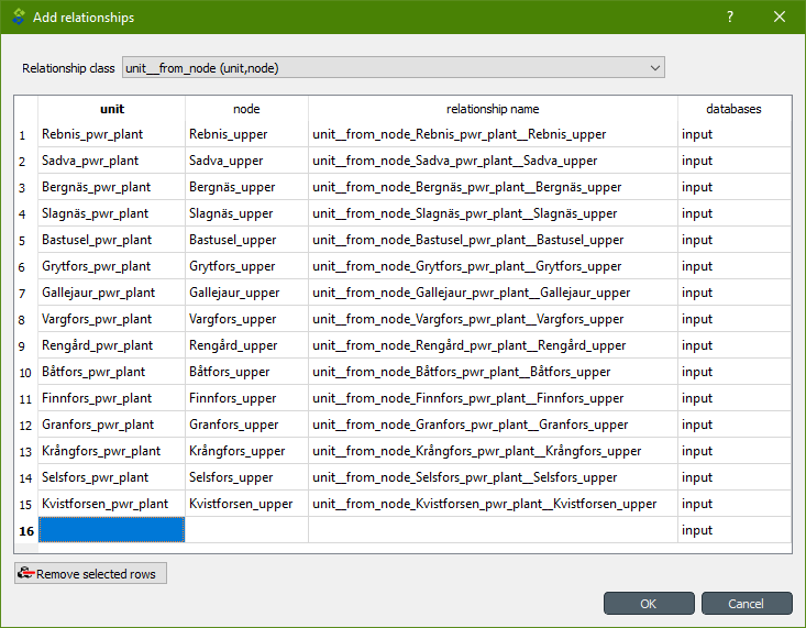
Click Ok.
Back in the Spine DB editor, under Relationship tree, double click on
unit__from_nodeto confirm that the relationships are effectively there.From the main menu, select Session -> Commit to open the Commit changes dialog. Enter ‘Add from nodes of power plants‘ as the commit message and click Commit.
Establish that (i) power plant units release water to the station’s lower node, and (ii) power plant units inject electricity to the common electricity node. Repeate the above procedure to create relationships of class
unit__to_nodewith the following data:Rebnis_pwr_plant Rebnis_lower Sadva_pwr_plant Sadva_lower Bergnäs_pwr_plant Bergnäs_lower Slagnäs_pwr_plant Slagnäs_lower Bastusel_pwr_plant Bastusel_lower Grytfors_pwr_plant Grytfors_lower Gallejaur_pwr_plant Gallejaur_lower Vargfors_pwr_plant Vargfors_lower Rengård_pwr_plant Rengård_lower Båtfors_pwr_plant Båtfors_lower Finnfors_pwr_plant Finnfors_lower Granfors_pwr_plant Granfors_lower Krångfors_pwr_plant Krångfors_lower Selsfors_pwr_plant Selsfors_lower Kvistforsen_pwr_plant Kvistforsen_lower Rebnis_pwr_plant electricity_node Sadva_pwr_plant electricity_node Bergnäs_pwr_plant electricity_node Slagnäs_pwr_plant electricity_node Bastusel_pwr_plant electricity_node Grytfors_pwr_plant electricity_node Gallejaur_pwr_plant electricity_node Vargfors_pwr_plant electricity_node Rengård_pwr_plant electricity_node Båtfors_pwr_plant electricity_node Finnfors_pwr_plant electricity_node Granfors_pwr_plant electricity_node Krångfors_pwr_plant electricity_node Selsfors_pwr_plant electricity_node Kvistforsen_pwr_plant electricity_node
Note
At this point, you might be wondering what’s the purpose of the
unit__node__noderelationship class. Shouldn’t it be enough to haveunit__from_nodeandunit__to_nodeto represent the topology of the system? The answer is yes; but in addition to topology, we also need to represent the conversion process that happens in the unit, where the water from one node is turned into electricty for another node. And for this purpose, we use a relationship parameter value on theunit__node__noderelationships (see Specifying relationship parameter values).Establish that (i) discharge connections take water from the lower node of the upstream station, and (ii) spillway connections take water from the upper node of the upstream station. Repeat the procedure to create relationships of class
connection__from_nodewith the following data:Bastusel_to_Grytfors_disch Bastusel_lower Bergnäs_to_Slagnäs_disch Bergnäs_lower Båtfors_to_Finnfors_disch Båtfors_lower Finnfors_to_Granfors_disch Finnfors_lower Gallejaur_to_Vargfors_disch Gallejaur_lower Granfors_to_Krångfors_disch Granfors_lower Grytfors_to_Gallejaur_disch Grytfors_lower Krångfors_to_Selsfors_disch Krångfors_lower Kvistforsen_to_downstream_disch Kvistforsen_lower Rebnis_to_Bergnäs_disch Rebnis_lower Rengård_to_Båtfors_disch Rengård_lower Sadva_to_Bergnäs_disch Sadva_lower Selsfors_to_Kvistforsen_disch Selsfors_lower Slagnäs_to_Bastusel_disch Slagnäs_lower Vargfors_to_Rengård_disch Vargfors_lower Bastusel_to_Grytfors_spill Bastusel_upper Bergnäs_to_Slagnäs_spill Bergnäs_upper Båtfors_to_Finnfors_spill Båtfors_upper Finnfors_to_Granfors_spill Finnfors_upper Gallejaur_to_Vargfors_spill Gallejaur_upper Granfors_to_Krångfors_spill Granfors_upper Grytfors_to_Gallejaur_spill Grytfors_upper Krångfors_to_Selsfors_spill Krångfors_upper Kvistforsen_to_downstream_spill Kvistforsen_upper Rebnis_to_Bergnäs_spill Rebnis_upper Rengård_to_Båtfors_spill Rengård_upper Sadva_to_Bergnäs_spill Sadva_upper Selsfors_to_Kvistforsen_spill Selsfors_upper Slagnäs_to_Bastusel_spill Slagnäs_upper Vargfors_to_Rengård_spill Vargfors_upper
Establish that both discharge and spillway connections release water onto the upper node of the downstream station. Repeat the procedure to create
connection__to_noderelationships with the following data:Bastusel_to_Grytfors_disch Grytfors_upper Bastusel_to_Grytfors_spill Grytfors_upper Bergnäs_to_Slagnäs_disch Slagnäs_upper Bergnäs_to_Slagnäs_spill Slagnäs_upper Båtfors_to_Finnfors_disch Finnfors_upper Båtfors_to_Finnfors_spill Finnfors_upper Finnfors_to_Granfors_disch Granfors_upper Finnfors_to_Granfors_spill Granfors_upper Gallejaur_to_Vargfors_disch Vargfors_upper Gallejaur_to_Vargfors_spill Vargfors_upper Granfors_to_Krångfors_disch Krångfors_upper Granfors_to_Krångfors_spill Krångfors_upper Grytfors_to_Gallejaur_disch Gallejaur_upper Grytfors_to_Gallejaur_spill Gallejaur_upper Krångfors_to_Selsfors_disch Selsfors_upper Krångfors_to_Selsfors_spill Selsfors_upper Rebnis_to_Bergnäs_disch Bergnäs_upper Rebnis_to_Bergnäs_spill Bergnäs_upper Rengård_to_Båtfors_disch Båtfors_upper Rengård_to_Båtfors_spill Båtfors_upper Sadva_to_Bergnäs_disch Bergnäs_upper Sadva_to_Bergnäs_spill Bergnäs_upper Selsfors_to_Kvistforsen_disch Kvistforsen_upper Selsfors_to_Kvistforsen_spill Kvistforsen_upper Slagnäs_to_Bastusel_disch Bastusel_upper Slagnäs_to_Bastusel_spill Bastusel_upper Vargfors_to_Rengård_disch Rengård_upper Vargfors_to_Rengård_spill Rengård_upper
Note
At this point, you might be wondering what’s the purpose of the
connection__node__noderelationship class. Shouldn’t it be enough to haveconnection__from_nodeandconnection__to_nodeto represent the topology of the system? The answer is yes; but in addition to topology, we also need to represent the delay in the river branches. And for this purpose, we use a relationship parameter value on theconnection__node__noderelationships (see Specifying relationship parameter values).Establish that water nodes balance water and the electricity node balances electricity. Repeat the procedure to create
node__commodityrelationships between all upper and lower reservoir nodes and thewatercommodity, as well as between theelectricity_nodeandelectricity.Rebnis_upper water Sadva_upper water Bergnäs_upper water Slagnäs_upper water Bastusel_upper water Grytfors_upper water Gallejaur_upper water Vargfors_upper water Rengård_upper water Båtfors_upper water Finnfors_upper water Granfors_upper water Krångfors_upper water Selsfors_upper water Kvistforsen_upper water Rebnis_lower water Sadva_lower water Bergnäs_lower water Slagnäs_lower water Bastusel_lower water Grytfors_lower water Gallejaur_lower water Vargfors_lower water Rengård_lower water Båtfors_lower water Finnfors_lower water Granfors_lower water Krångfors_lower water Selsfors_lower water Kvistforsen_lower water electricity_node electricity
Establish that all nodes are balanced at each time slice in the one week horizon. Create relationships of class
model__default_temporal_blockbetween the modelinstanceand the temporal_blocksome_week.Establish that this model is deterministic. Create a relationships of class
model__default_stochastic_structurebetween the modelinstanceanddeterministic, and a relationship of classstochastic_structure__stochastic_scenariobetweendeterministicandrealization.Finally, create one relationship of class
report__outputbetweenmy_reportand each of the followingoutputobjects:unit_flow,connection_flow, andnode_state, as well as one relationship of classmodel__reportbetweeninstanceandmy_report. This is so results from running Spine Opt are written to the ouput database.
Specifying relationship parameter values
Specify (i) the capacity of hydro power plants, and (ii) the variable operating cost of the electricity unit (equal to the negative electricity price). Enter
unit__from_nodeparameter values as follows:Select the parameter value data from the text-box below and copy it to the clipboard (Ctrl+C):
unit__from_node	Bastusel_pwr_plant,Bastusel_upper	unit_capacity	Base	127.5
unit__from_node	Bergnäs_pwr_plant,Bergnäs_upper	unit_capacity	Base	120
unit__from_node	Båtfors_pwr_plant,Båtfors_upper	unit_capacity	Base	210
unit__from_node	Finnfors_pwr_plant,Finnfors_upper	unit_capacity	Base	176.25
unit__from_node	Gallejaur_pwr_plant,Gallejaur_upper	unit_capacity	Base	228.75
unit__from_node	Granfors_pwr_plant,Granfors_upper	unit_capacity	Base	180
unit__from_node	Grytfors_pwr_plant,Grytfors_upper	unit_capacity	Base	123.75
unit__from_node	Krångfors_pwr_plant,Krångfors_upper	unit_capacity	Base	180
unit__from_node	Kvistforsen_pwr_plant,Kvistforsen_upper	minimum_operating_point	Base	0.0888888888889
unit__from_node	Kvistforsen_pwr_plant,Kvistforsen_upper	unit_capacity	Base	225
unit__from_node	Rebnis_pwr_plant,Rebnis_upper	unit_capacity	Base	60
unit__from_node	Rengård_pwr_plant,Rengård_upper	unit_capacity	Base	165
unit__from_node	Sadva_pwr_plant,Sadva_upper	unit_capacity	Base	52.5
unit__from_node	Selsfors_pwr_plant,Selsfors_upper	unit_capacity	Base	225
unit__from_node	Slagnäs_pwr_plant,Slagnäs_upper	unit_capacity	Base	120
unit__from_node	Vargfors_pwr_plant,Vargfors_upper	unit_capacity	Base	232.5
unit__from_node	electricity_load,electricity_node	vom_cost	Base	{"type": "time_series", "index": {"start": "2019-01-01 00:00:00", "resolution": "1h", "ignore_year": false, "repeat": false}, "data": [-162.03, -156.36, -151.06, -153.52, -158.91, -164.02, -175.56, -283.11, -278.76, -299.57, -285.28, -207.34, -194.95, -190.41, -185.4, -183.41, -191.54, -202.9, -197.69, -195.33, -186.72, -178.87, -174.71, -168.75, -172.89, -172.13, -171.66, -173.27, -176.97, -179.63, -226.41, -271.96, -399.3, -402.53, -353.28, -330.79, -294.54, -271.29, -248.71, -226.79, -240.93, -374.44, -255.54, -210.47, -186.65, -178.21, -173.18, -166.44, -165.09, -162.91, -161.11, -162.53, -166.04, -169.16, -174.28, -185.37, -195.79, -189.92, -187.74, -181.96, -179.12, -178.36, -177.13, -177.03, -177.69, -184.8, -187.27, -179.49, -175.23, -172.67, -169.07, -165.37, -170.06, -171.48, -171.58, -174.14, -180.3, -185.89, -195.37, -328.65, -365.91, -315.0, -242.68, -230.73, -225.33, -225.8, -213.38, -207.32, -215.37, -243.81, -243.53, -215.56, -192.05, -187.88, -181.15, -172.15, -174.16, -171.05, -170.77, -174.82, -179.62, -178.87, -191.49, -229.64, -336.07, -242.07, -228.5, -201.85, -196.67, -192.34, -190.36, -187.44, -186.68, -190.26, -191.21, -187.53, -179.34, -171.9, -166.53, -160.59, -166.08, -157.74, -145.36, -145.64, -147.42, -149.77, -153.33, -141.33, -145.08, -150.52, -153.42, -159.43, -159.05, -149.49, -147.89, -150.52, -157.08, -172.37, -174.06, -171.15, -160.46, -147.8, -141.61, -134.39, -144.41, -140.19, -138.59, -140.0, -139.53, -140.28, -144.03, -146.57, -149.39, -156.24, -157.93, -156.43, -155.21, -149.86, -148.07, -147.13, -148.82, -162.53, -174.74, -170.89, -163.94, -157.93, -150.7, -143.94]}
Go to Relationship parameter value (on the bottom-center of the window, usually). Make sure that the columns in the table are ordered as follows:
relationship_class_name | object_name_list | parameter_name | alternative_name | value | database
Select the first empty cell under
relationship_class_nameand press Ctrl+V. This will paste the parameter value data from the clipboard into the table.
Specify the conversion ratio from water to electricity and from water to water of different hydro power plants (the latter being equal to 1). Repeat the same procedure with the data below:
unit__node__node	Bastusel_pwr_plant,electricity_node,Bastusel_upper	fix_ratio_out_in_unit_flow	Base	0.577810871184
unit__node__node	Bergnäs_pwr_plant,electricity_node,Bergnäs_upper	fix_ratio_out_in_unit_flow	Base	0.0506329113924
unit__node__node	Båtfors_pwr_plant,electricity_node,Båtfors_upper	fix_ratio_out_in_unit_flow	Base	0.148282097649
unit__node__node	Finnfors_pwr_plant,electricity_node,Finnfors_upper	fix_ratio_out_in_unit_flow	Base	0.180985725828
unit__node__node	Gallejaur_pwr_plant,electricity_node,Gallejaur_upper	fix_ratio_out_in_unit_flow	Base	0.730442000415
unit__node__node	Granfors_pwr_plant,electricity_node,Granfors_upper	fix_ratio_out_in_unit_flow	Base	0.164556962025
unit__node__node	Grytfors_pwr_plant,electricity_node,Grytfors_upper	fix_ratio_out_in_unit_flow	Base	0.190257000384
unit__node__node	Krångfors_pwr_plant,electricity_node,Krångfors_upper	fix_ratio_out_in_unit_flow	Base	0.274261603376
unit__node__node	Kvistforsen_pwr_plant,electricity_node,Kvistforsen_upper	fix_ratio_out_in_unit_flow	Base	0.472573839662
unit__node__node	Rebnis_pwr_plant,electricity_node,Rebnis_upper	fix_ratio_out_in_unit_flow	Base	0.810126582278
unit__node__node	Rengård_pwr_plant,electricity_node,Rengård_upper	fix_ratio_out_in_unit_flow	Base	0.165707710012
unit__node__node	Sadva_pwr_plant,electricity_node,Sadva_upper	fix_ratio_out_in_unit_flow	Base	0.448462929476
unit__node__node	Selsfors_pwr_plant,electricity_node,Selsfors_upper	fix_ratio_out_in_unit_flow	Base	0.209282700422
unit__node__node	Slagnäs_pwr_plant,electricity_node,Slagnäs_upper	fix_ratio_out_in_unit_flow	Base	0.0443037974684
unit__node__node	Vargfors_pwr_plant,electricity_node,Vargfors_upper	fix_ratio_out_in_unit_flow	Base	0.34299714169
unit__node__node	Bastusel_pwr_plant,Bastusel_lower,Bastusel_upper	fix_ratio_out_in_unit_flow	Base	1
unit__node__node	Bergnäs_pwr_plant,Bergnäs_lower,Bergnäs_upper	fix_ratio_out_in_unit_flow	Base	1
unit__node__node	Båtfors_pwr_plant,Båtfors_lower,Båtfors_upper	fix_ratio_out_in_unit_flow	Base	1
unit__node__node	Finnfors_pwr_plant,Finnfors_lower,Finnfors_upper	fix_ratio_out_in_unit_flow	Base	1
unit__node__node	Gallejaur_pwr_plant,Gallejaur_lower,Gallejaur_upper	fix_ratio_out_in_unit_flow	Base	1
unit__node__node	Granfors_pwr_plant,Granfors_lower,Granfors_upper	fix_ratio_out_in_unit_flow	Base	1
unit__node__node	Grytfors_pwr_plant,Grytfors_lower,Grytfors_upper	fix_ratio_out_in_unit_flow	Base	1
unit__node__node	Krångfors_pwr_plant,Krångfors_lower,Krångfors_upper	fix_ratio_out_in_unit_flow	Base	1
unit__node__node	Kvistforsen_pwr_plant,Kvistforsen_lower,Kvistforsen_upper	fix_ratio_out_in_unit_flow	Base	1
unit__node__node	Rebnis_pwr_plant,Rebnis_lower,Rebnis_upper	fix_ratio_out_in_unit_flow	Base	1
unit__node__node	Rengård_pwr_plant,Rengård_lower,Rengård_upper	fix_ratio_out_in_unit_flow	Base	1
unit__node__node	Sadva_pwr_plant,Sadva_lower,Sadva_upper	fix_ratio_out_in_unit_flow	Base	1
unit__node__node	Selsfors_pwr_plant,Selsfors_lower,Selsfors_upper	fix_ratio_out_in_unit_flow	Base	1
unit__node__node	Slagnäs_pwr_plant,Slagnäs_lower,Slagnäs_upper	fix_ratio_out_in_unit_flow	Base	1
unit__node__node	Vargfors_pwr_plant,Vargfors_lower,Vargfors_upper	fix_ratio_out_in_unit_flow	Base	1
specify the average discharge and spillage in the first hours of the simulation. Repeat the same procedure with the data below:
connection__from_node	Bastusel_to_Grytfors_disch,Bastusel_lower	fix_connection_flow	Base	{"type": "time_series", "index": {"start": "2018-12-30 00:00:00", "resolution": "2D"}, "data": [110.7, 110.7]}
connection__from_node	Bergnäs_to_Slagnäs_disch,Bergnäs_lower	fix_connection_flow	Base	{"type": "time_series", "index": {"start": "2018-12-30 00:00:00", "resolution": "2D"}, "data": [105.0, 105.0]}
connection__from_node	Båtfors_to_Finnfors_disch,Båtfors_lower	fix_connection_flow	Base	{"type": "time_series", "index": {"start": "2018-12-30 00:00:00", "resolution": "2D"}, "data": [150.2, 150.2]}
connection__from_node	Finnfors_to_Granfors_disch,Finnfors_lower	fix_connection_flow	Base	{"type": "time_series", "index": {"start": "2018-12-30 00:00:00", "resolution": "2D"}, "data": [155.3, 155.3]}
connection__from_node	Gallejaur_to_Vargfors_disch,Gallejaur_lower	fix_connection_flow	Base	{"type": "time_series", "index": {"start": "2018-12-30 00:00:00", "resolution": "2D"}, "data": [118.2, 118.2]}
connection__from_node	Granfors_to_Krångfors_disch,Granfors_lower	fix_connection_flow	Base	{"type": "time_series", "index": {"start": "2018-12-30 00:00:00", "resolution": "2D"}, "data": [155.6, 155.6]}
connection__from_node	Grytfors_to_Gallejaur_disch,Grytfors_lower	fix_connection_flow	Base	{"type": "time_series", "index": {"start": "2018-12-30 00:00:00", "resolution": "2D"}, "data": [117.2, 117.2]}
connection__from_node	Krångfors_to_Selsfors_disch,Krångfors_lower	fix_connection_flow	Base	{"type": "time_series", "index": {"start": "2018-12-30 00:00:00", "resolution": "2D"}, "data": [156.0, 156.0]}
connection__from_node	Kvistforsen_to_downstream_disch,Kvistforsen_lower	fix_connection_flow	Base	{"type": "time_series", "index": {"start": "2018-12-30 00:00:00", "resolution": "2D"}, "data": [158.5, 158.5]}
connection__from_node	Rebnis_to_Bergnäs_disch,Rebnis_lower	fix_connection_flow	Base	{"type": "time_series", "index": {"start": "2018-12-30 00:00:00", "resolution": "2D"}, "data": [21.5, 21.5]}
connection__from_node	Rengård_to_Båtfors_disch,Rengård_lower	fix_connection_flow	Base	{"type": "time_series", "index": {"start": "2018-12-30 00:00:00", "resolution": "2D"}, "data": [141.5, 141.5]}
connection__from_node	Sadva_to_Bergnäs_disch,Sadva_lower	fix_connection_flow	Base	{"type": "time_series", "index": {"start": "2018-12-30 00:00:00", "resolution": "2D"}, "data": [34.6, 34.6]}
connection__from_node	Selsfors_to_Kvistforsen_disch,Selsfors_lower	fix_connection_flow	Base	{"type": "time_series", "index": {"start": "2018-12-30 00:00:00", "resolution": "2D"}, "data": [158.4, 158.4]}
connection__from_node	Slagnäs_to_Bastusel_disch,Slagnäs_lower	fix_connection_flow	Base	{"type": "time_series", "index": {"start": "2018-12-30 00:00:00", "resolution": "2D"}, "data": [106.6, 106.6]}
connection__from_node	Vargfors_to_Rengård_disch,Vargfors_lower	fix_connection_flow	Base	{"type": "time_series", "index": {"start": "2018-12-30 00:00:00", "resolution": "2D"}, "data": [119.6, 119.6]}
connection__from_node	Bastusel_to_Grytfors_spill,Bastusel_upper	fix_connection_flow	Base	{"type": "time_series", "index": {"start": "2018-12-30 00:00:00", "resolution": "2D"}, "data": [0.0, 0.0]}
connection__from_node	Bergnäs_to_Slagnäs_spill,Bergnäs_upper	fix_connection_flow	Base	{"type": "time_series", "index": {"start": "2018-12-30 00:00:00", "resolution": "2D"}, "data": [0.0, 0.0]}
connection__from_node	Båtfors_to_Finnfors_spill,Båtfors_upper	fix_connection_flow	Base	{"type": "time_series", "index": {"start": "2018-12-30 00:00:00", "resolution": "2D"}, "data": [0.0, 0.0]}
connection__from_node	Finnfors_to_Granfors_spill,Finnfors_upper	fix_connection_flow	Base	{"type": "time_series", "index": {"start": "2018-12-30 00:00:00", "resolution": "2D"}, "data": [0.0, 0.0]}
connection__from_node	Gallejaur_to_Vargfors_spill,Gallejaur_upper	fix_connection_flow	Base	{"type": "time_series", "index": {"start": "2018-12-30 00:00:00", "resolution": "2D"}, "data": [0.0, 0.0]}
connection__from_node	Granfors_to_Krångfors_spill,Granfors_upper	fix_connection_flow	Base	{"type": "time_series", "index": {"start": "2018-12-30 00:00:00", "resolution": "2D"}, "data": [0.0, 0.0]}
connection__from_node	Grytfors_to_Gallejaur_spill,Grytfors_upper	fix_connection_flow	Base	{"type": "time_series", "index": {"start": "2018-12-30 00:00:00", "resolution": "2D"}, "data": [0.0, 0.0]}
connection__from_node	Krångfors_to_Selsfors_spill,Krångfors_upper	fix_connection_flow	Base	{"type": "time_series", "index": {"start": "2018-12-30 00:00:00", "resolution": "2D"}, "data": [0.0, 0.0]}
connection__from_node	Kvistforsen_to_downstream_spill,Kvistforsen_upper	fix_connection_flow	Base	{"type": "time_series", "index": {"start": "2018-12-30 00:00:00", "resolution": "2D"}, "data": [0.0, 0.0]}
connection__from_node	Rebnis_to_Bergnäs_spill,Rebnis_upper	fix_connection_flow	Base	{"type": "time_series", "index": {"start": "2018-12-30 00:00:00", "resolution": "2D"}, "data": [0.0, 0.0]}
connection__from_node	Rengård_to_Båtfors_spill,Rengård_upper	fix_connection_flow	Base	{"type": "time_series", "index": {"start": "2018-12-30 00:00:00", "resolution": "2D"}, "data": [0.0, 0.0]}
connection__from_node	Sadva_to_Bergnäs_spill,Sadva_upper	fix_connection_flow	Base	{"type": "time_series", "index": {"start": "2018-12-30 00:00:00", "resolution": "2D"}, "data": [0.0, 0.0]}
connection__from_node	Selsfors_to_Kvistforsen_spill,Selsfors_upper	fix_connection_flow	Base	{"type": "time_series", "index": {"start": "2018-12-30 00:00:00", "resolution": "2D"}, "data": [0.0, 0.0]}
connection__from_node	Slagnäs_to_Bastusel_spill,Slagnäs_upper	fix_connection_flow	Base	{"type": "time_series", "index": {"start": "2018-12-30 00:00:00", "resolution": "2D"}, "data": [0.0, 0.0]}
connection__from_node	Vargfors_to_Rengård_spill,Vargfors_upper	fix_connection_flow	Base	{"type": "time_series", "index": {"start": "2018-12-30 00:00:00", "resolution": "2D"}, "data": [0.0, 0.0]}
Finally, specify the delay and transfer ratio of different water connections (the latter being equal to 1). Repeat the same procedure with the data below:
connection__node__node	Bastusel_to_Grytfors_disch,Grytfors_upper,Bastusel_lower	connection_flow_delay	Base	{"type": "duration", "data": "1h"}
connection__node__node	Bastusel_to_Grytfors_spill,Grytfors_upper,Bastusel_upper	connection_flow_delay	Base	{"type": "duration", "data": "150m"}
connection__node__node	Bergnäs_to_Slagnäs_disch,Slagnäs_upper,Bergnäs_lower	connection_flow_delay	Base	{"type": "duration", "data": "1h"}
connection__node__node	Bergnäs_to_Slagnäs_spill,Slagnäs_upper,Bergnäs_upper	connection_flow_delay	Base	{"type": "duration", "data": "1h"}
connection__node__node	Båtfors_to_Finnfors_disch,Finnfors_upper,Båtfors_lower	connection_flow_delay	Base	{"type": "duration", "data": "3h"}
connection__node__node	Båtfors_to_Finnfors_spill,Finnfors_upper,Båtfors_upper	connection_flow_delay	Base	{"type": "duration", "data": "3h"}
connection__node__node	Finnfors_to_Granfors_disch,Granfors_upper,Finnfors_lower	connection_flow_delay	Base	{"type": "duration", "data": "3h"}
connection__node__node	Finnfors_to_Granfors_spill,Granfors_upper,Finnfors_upper	connection_flow_delay	Base	{"type": "duration", "data": "3h"}
connection__node__node	Gallejaur_to_Vargfors_disch,Vargfors_upper,Gallejaur_lower	connection_flow_delay	Base	{"type": "duration", "data": "30m"}
connection__node__node	Gallejaur_to_Vargfors_spill,Vargfors_upper,Gallejaur_upper	connection_flow_delay	Base	{"type": "duration", "data": "150m"}
connection__node__node	Granfors_to_Krångfors_disch,Krångfors_upper,Granfors_lower	connection_flow_delay	Base	{"type": "duration", "data": "3h"}
connection__node__node	Granfors_to_Krångfors_spill,Krångfors_upper,Granfors_upper	connection_flow_delay	Base	{"type": "duration", "data": "3h"}
connection__node__node	Grytfors_to_Gallejaur_disch,Gallejaur_upper,Grytfors_lower	connection_flow_delay	Base	{"type": "duration", "data": "15m"}
connection__node__node	Grytfors_to_Gallejaur_spill,Gallejaur_upper,Grytfors_upper	connection_flow_delay	Base	{"type": "duration", "data": "15m"}
connection__node__node	Krångfors_to_Selsfors_disch,Selsfors_upper,Krångfors_lower	connection_flow_delay	Base	{"type": "duration", "data": "3h"}
connection__node__node	Krångfors_to_Selsfors_spill,Selsfors_upper,Krångfors_upper	connection_flow_delay	Base	{"type": "duration", "data": "3h"}
connection__node__node	Rebnis_to_Bergnäs_disch,Bergnäs_upper,Rebnis_lower	connection_flow_delay	Base	{"type": "duration", "data": "2D"}
connection__node__node	Rebnis_to_Bergnäs_spill,Bergnäs_upper,Rebnis_upper	connection_flow_delay	Base	{"type": "duration", "data": "2D"}
connection__node__node	Rengård_to_Båtfors_disch,Båtfors_upper,Rengård_lower	connection_flow_delay	Base	{"type": "duration", "data": "3h"}
connection__node__node	Rengård_to_Båtfors_spill,Båtfors_upper,Rengård_upper	connection_flow_delay	Base	{"type": "duration", "data": "3h"}
connection__node__node	Sadva_to_Bergnäs_disch,Bergnäs_upper,Sadva_lower	connection_flow_delay	Base	{"type": "duration", "data": "2D"}
connection__node__node	Sadva_to_Bergnäs_spill,Bergnäs_upper,Sadva_upper	connection_flow_delay	Base	{"type": "duration", "data": "2D"}
connection__node__node	Selsfors_to_Kvistforsen_disch,Kvistforsen_upper,Selsfors_lower	connection_flow_delay	Base	{"type": "duration", "data": "3h"}
connection__node__node	Selsfors_to_Kvistforsen_spill,Kvistforsen_upper,Selsfors_upper	connection_flow_delay	Base	{"type": "duration", "data": "3h"}
connection__node__node	Slagnäs_to_Bastusel_disch,Bastusel_upper,Slagnäs_lower	connection_flow_delay	Base	{"type": "duration", "data": "4h"}
connection__node__node	Slagnäs_to_Bastusel_spill,Bastusel_upper,Slagnäs_upper	connection_flow_delay	Base	{"type": "duration", "data": "4h"}
connection__node__node	Vargfors_to_Rengård_disch,Rengård_upper,Vargfors_lower	connection_flow_delay	Base	{"type": "duration", "data": "3h"}
connection__node__node	Vargfors_to_Rengård_spill,Rengård_upper,Vargfors_upper	connection_flow_delay	Base	{"type": "duration", "data": "3h"}
connection__node__node	Bastusel_to_Grytfors_disch,Grytfors_upper,Bastusel_lower	fix_ratio_out_in_connection_flow	Base	1
connection__node__node	Bastusel_to_Grytfors_spill,Grytfors_upper,Bastusel_upper	fix_ratio_out_in_connection_flow	Base	1
connection__node__node	Bergnäs_to_Slagnäs_disch,Slagnäs_upper,Bergnäs_lower	fix_ratio_out_in_connection_flow	Base	1
connection__node__node	Bergnäs_to_Slagnäs_spill,Slagnäs_upper,Bergnäs_upper	fix_ratio_out_in_connection_flow	Base	1
connection__node__node	Båtfors_to_Finnfors_disch,Finnfors_upper,Båtfors_lower	fix_ratio_out_in_connection_flow	Base	1
connection__node__node	Båtfors_to_Finnfors_spill,Finnfors_upper,Båtfors_upper	fix_ratio_out_in_connection_flow	Base	1
connection__node__node	Finnfors_to_Granfors_disch,Granfors_upper,Finnfors_lower	fix_ratio_out_in_connection_flow	Base	1
connection__node__node	Finnfors_to_Granfors_spill,Granfors_upper,Finnfors_upper	fix_ratio_out_in_connection_flow	Base	1
connection__node__node	Gallejaur_to_Vargfors_disch,Vargfors_upper,Gallejaur_lower	fix_ratio_out_in_connection_flow	Base	1
connection__node__node	Gallejaur_to_Vargfors_spill,Vargfors_upper,Gallejaur_upper	fix_ratio_out_in_connection_flow	Base	1
connection__node__node	Granfors_to_Krångfors_disch,Krångfors_upper,Granfors_lower	fix_ratio_out_in_connection_flow	Base	1
connection__node__node	Granfors_to_Krångfors_spill,Krångfors_upper,Granfors_upper	fix_ratio_out_in_connection_flow	Base	1
connection__node__node	Grytfors_to_Gallejaur_disch,Gallejaur_upper,Grytfors_lower	fix_ratio_out_in_connection_flow	Base	1
connection__node__node	Grytfors_to_Gallejaur_spill,Gallejaur_upper,Grytfors_upper	fix_ratio_out_in_connection_flow	Base	1
connection__node__node	Krångfors_to_Selsfors_disch,Selsfors_upper,Krångfors_lower	fix_ratio_out_in_connection_flow	Base	1
connection__node__node	Krångfors_to_Selsfors_spill,Selsfors_upper,Krångfors_upper	fix_ratio_out_in_connection_flow	Base	1
connection__node__node	Rebnis_to_Bergnäs_disch,Bergnäs_upper,Rebnis_lower	fix_ratio_out_in_connection_flow	Base	1
connection__node__node	Rebnis_to_Bergnäs_spill,Bergnäs_upper,Rebnis_upper	fix_ratio_out_in_connection_flow	Base	1
connection__node__node	Rengård_to_Båtfors_disch,Båtfors_upper,Rengård_lower	fix_ratio_out_in_connection_flow	Base	1
connection__node__node	Rengård_to_Båtfors_spill,Båtfors_upper,Rengård_upper	fix_ratio_out_in_connection_flow	Base	1
connection__node__node	Sadva_to_Bergnäs_disch,Bergnäs_upper,Sadva_lower	fix_ratio_out_in_connection_flow	Base	1
connection__node__node	Sadva_to_Bergnäs_spill,Bergnäs_upper,Sadva_upper	fix_ratio_out_in_connection_flow	Base	1
connection__node__node	Selsfors_to_Kvistforsen_disch,Kvistforsen_upper,Selsfors_lower	fix_ratio_out_in_connection_flow	Base	1
connection__node__node	Selsfors_to_Kvistforsen_spill,Kvistforsen_upper,Selsfors_upper	fix_ratio_out_in_connection_flow	Base	1
connection__node__node	Slagnäs_to_Bastusel_disch,Bastusel_upper,Slagnäs_lower	fix_ratio_out_in_connection_flow	Base	1
connection__node__node	Slagnäs_to_Bastusel_spill,Bastusel_upper,Slagnäs_upper	fix_ratio_out_in_connection_flow	Base	1
connection__node__node	Vargfors_to_Rengård_disch,Rengård_upper,Vargfors_lower	fix_ratio_out_in_connection_flow	Base	1
connection__node__node	Vargfors_to_Rengård_spill,Rengård_upper,Vargfors_upper	fix_ratio_out_in_connection_flow	Base	1
When you’re ready, commit all changes to the database.
Executing the workflow
Once the workflow is defined and input data is in place, the project is ready
to be executed. Hit the Execute project button ![]() on
the tool bar.
on
the tool bar.
You should see ‘Executing All Directed Acyclic Graphs’ printed in the Event log (on the lower left by default). SpineOpt output messages will appear in the Process Log panel in the middle. After some processing, ‘DAG 1/1 completed successfully’ appears and the execution is complete.
Examining the results
Select the output data store and open the Spine DB editor.
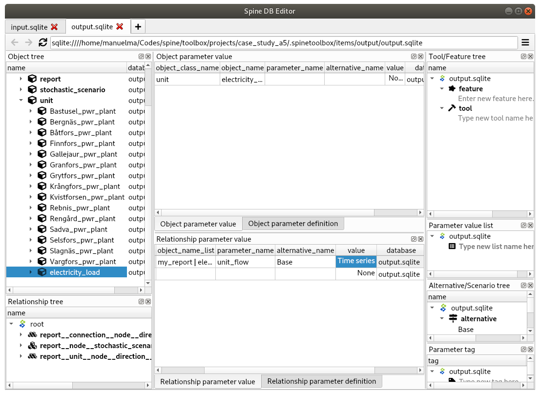
To checkout the flow on the electricity load (i.e., the total electricity production in the system),
go to Object tree, expand the unit object class,
and select electricity_load, as illustrated in the picture above.
Next, go to Relationship parameter value and double-click the first cell under value.
The Parameter value editor will pop up. You should see something like this:
