Case Study A5 tutorial

Welcome to Spine Toolbox’s Case Study A5 tutorial. Case Study A5 is one of the Spine Project case studies designed to verify Toolbox and Model capabilities. To this end, it reproduces an already existing study about hydropower on the Skellefte river, which models one week of operation of the fifteen power stations along the river.

This tutorial provides a step-by-step guide to run Case Study A5 on Spine Toolbox and is organized as follows:

Introduction

Model assumptions

For each power station in the river, the following information is known:

• The capacity, or maximum electricity output. This datum also provides the maximum water discharge as per the efficiency curve (see next point).
• The efficiency curve, or conversion rate from water to electricity. In this study, a piece-wise linear efficiency with two segments is assumed. Moreover, this curve is monotonically decreasing, i.e., the efficiency in the first segment is strictly greater than the efficiency in the second segment.
• The maximum magazine level, or amount of water that can be stored in the reservoir.
• The magazine level at the beginning of the simulation period, and at the end.
• The minimum amount of water that the plant needs to discharge at every hour. This is usually zero (except for one of the plants).
• The minimum amount of water that needs to be spilled at every hour. Spilled water does not go through the turbine and thus does not serve to produce electricity; it just helps keeping the magazine level at bay.
• The downstream plant, or next plant in the river course.
• The time that it takes for the water to reach the downstream plant. This time can be different depending on whether the water is discharged (goes through the turbine) or spilled.
• The local inflow, or amount of water that naturally enters the reservoir at every hour. In this study, it is assumed constant over the entire simulation period.
• The hourly average water discharge. It is assumed that before the beginning of the simulation, this amount of water has constantly been discharged at every hour.

The system is operated so as to maximize total profit over the week, while respecting capacity constraints, maximum magazine level constrains, and so on. Hourly profit per plant is simply computed as the product of the electricity price and the production, minus a penalty for changes on the water discharge in two consecutive hours. This penalty is computed as the product of a constant penalty factor, common to all plants, and the absolute value of the difference in discharge with respect to the previous hour.

Modelling choices

The model of the electric system is fairly simple, only two elements are needed:

• A common electricity node.
• A load unit that takes electricity from that node.

On the contrary, the model of the river system is more detailed. Each power station in the river is modelled using the following elements:

• An upper water node, located at the entrance of the station.
• A lower water node, located at the exit of the station.
• A reservoir unit, that takes water from the upper node to put it into a water storage and viceversa.
• A power plant unit, that discharges water from the upper node into the lower node, and feeds electricity produced in the process to the common electricity node.
• A spillway connection, that takes spilled water from the upper node and releases it to the downstream upper node.
• A discharge connection, that takes water from the lower node and releases it to the downstream upper node.

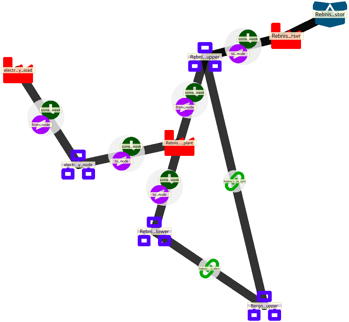
Below is a schematic of the model. For clarity, only the Rebnis station is presented in full detail:

Guide

Installing requirements

Make sure that Spine Toolbox and julia 1.0 (or greater) are properly installed as described at the following links:

• Running Spine Toolbox
• Julia downloads

Setting up project

1. Launch Spine Toolbox and from the main menu, select File -> New… to create a new project. Type “Case Study A5” as the project name and click Ok.

2. Drag the Data Store icon () from the toolbar and drop it into the Design View. This will open the Add Data Store dialog. Type “input” as the Data Store name and click Ok.

3. Repeat the above operation to create a Data Store called “output”.

4. Drag the Tool icon () from the toolbar and drop it into the Design View. This will open the Add Tool dialog. Type “Spine model” as the Tool name and click Ok.

   Note

   Each item in the Design view is equipped with three connectors (the small squares at the item boundaries).

5. Click on one of “input” connectors and then on one of “Spine model” connectors. This will create a connection from the former to the latter.

6. Repeat the procedure to create a connection from “Spine model” to “output”. It should look something like this:

   Todo

   Add image

7. From the main menu, select File -> Save project.

Entering input data

Creating input database

1. Follow the steps below to create a new Spine database for Spine Model in the ‘input’ Data Store:

   1. Select the ‘input’ Data Store item in the Design View.
   2. Go to Data Store Properties, check the box that reads For Spine Model and press New Spine db.

2. Still in Data Store Properties, click Tree view. This will open the newly created database in the Data store tree view, looking similar to this:

   
   
   

   Note

   The Data store tree view is a dedicated interface within Spine Toolbox for visualizing and managing Spine databases.

Creating objects

1. Follow the steps below to add power plants to the model as objects of class unit:

   1. Go to Object tree, right-click on unit and select Add objects from the context menu. This will open the Add objects dialog.

   2. With your mouse, select the list of plant names from the text-box below and copy it to the clipboard (Ctrl+C):

      Rebnis_pwr_plant
      Sadva_pwr_plant
      Bergnäs_pwr_plant
      Slagnäs_pwr_plant
      Bastusel_pwr_plant
      Grytfors_pwr_plant
      Gallejaur_pwr_plant
      Vargfors_pwr_plant
      Rengård_pwr_plant
      Båtfors_pwr_plant
      Finnfors_pwr_plant
      Granfors_pwr_plant
      Krångfors_pwr_plant
      Selsfors_pwr_plant
      Kvistforsen_pwr_plant
      

   3. Go back to the Add objects dialog, select the first cell under the object name column and press Ctrl+V. This will paste the list of plant names from the clipboard into that column, looking similar to this:

      

   4. Click Ok.

   5. Back in the Data store tree view, under Object tree, double click on unit to confirm that the objects are effectively there.

   6. From the main menu, select Session -> Commit to open the Commit changes dialog. Enter “Add power plants” as the commit message and click Commit.

2. Repeat the procedure to add reservoirs as objects of class unit, with the following names:

   Rebnis_rsrv
   Sadva_rsrv
   Bergnäs_rsrv
   Slagnäs_rsrv
   Bastusel_rsrv
   Grytfors_rsrv
   Gallejaur_rsrv
   Vargfors_rsrv
   Rengård_rsrv
   Båtfors_rsrv
   Finnfors_rsrv
   Granfors_rsrv
   Krångfors_rsrv
   Selsfors_rsrv
   Kvistforsen_rsrv
   

3. Repeat the procedure to add discharge and spillway connections as objects of class connection, with the following names:

   Rebnis_to_Bergnäs_disch
   Sadva_to_Bergnäs_disch
   Bergnäs_to_Slagnäs_disch
   Slagnäs_to_Bastusel_disch
   Bastusel_to_Grytfors_disch
   Grytfors_to_Gallejaur_disch
   Gallejaur_to_Vargfors_disch
   Vargfors_to_Rengård_disch
   Rengård_to_Båtfors_disch
   Båtfors_to_Finnfors_disch
   Finnfors_to_Granfors_disch
   Granfors_to_Krångfors_disch
   Krångfors_to_Selsfors_disch
   Selsfors_to_Kvistforsen_disch
   Kvistforsen_to_downstream_disch
   Rebnis_to_Bergnäs_spill
   Sadva_to_Bergnäs_spill
   Bergnäs_to_Slagnäs_spill
   Slagnäs_to_Bastusel_spill
   Bastusel_to_Grytfors_spill
   Grytfors_to_Gallejaur_spill
   Gallejaur_to_Vargfors_spill
   Vargfors_to_Rengård_spill
   Rengård_to_Båtfors_spill
   Båtfors_to_Finnfors_spill
   Finnfors_to_Granfors_spill
   Granfors_to_Krångfors_spill
   Krångfors_to_Selsfors_spill
   Selsfors_to_Kvistforsen_spill
   Kvistforsen_to_downstream_spill
   

4. Repeat the procedure to add water storages as objects of class storage, with the following names:

   Rebnis_stor
   Sadva_stor
   Bergnäs_stor
   Slagnäs_stor
   Bastusel_stor
   Grytfors_stor
   Gallejaur_stor
   Vargfors_stor
   Rengård_stor
   Båtfors_stor
   Finnfors_stor
   Granfors_stor
   Krångfors_stor
   Selsfors_stor
   Kvistforsen_stor
   

5. Repeat the procedure to add water nodes as objects of class node, with the following names:

   Rebnis_upper
   Sadva_upper
   Bergnäs_upper
   Slagnäs_upper
   Bastusel_upper
   Grytfors_upper
   Gallejaur_upper
   Vargfors_upper
   Rengård_upper
   Båtfors_upper
   Finnfors_upper
   Granfors_upper
   Krångfors_upper
   Selsfors_upper
   Kvistforsen_upper
   Rebnis_lower
   Sadva_lower
   Bergnäs_lower
   Slagnäs_lower
   Bastusel_lower
   Grytfors_lower
   Gallejaur_lower
   Vargfors_lower
   Rengård_lower
   Båtfors_lower
   Finnfors_lower
   Granfors_lower
   Krångfors_lower
   Selsfors_lower
   Kvistforsen_lower
   

6. Finally, add water and electricity as objects of class commodity; electricity_node as an object of clas node; electricity_load as an object of class unit; and some_week and past as objects of class temporal_block.

Specifying object parameter values

TODO

Establishing relationships

1. Follow the steps below to establish that power plant units receive water from the station’s upper node at each time slice in the one week horizon, as relationships of class unit__node__direction__temporal_block:

   1. Go to Relationship tree, right-click on unit__node__direction__temporal_block and select Add relationships from the context menu. This will open the Add relationships dialog.

   2. Select again all power plant names and copy them to the clipboard (Ctrl+C).

   3. Go back to the Add relationships dialog, select the first cell under the unit name column and press Ctrl+V. This will paste the list of plant names from the clipboard into that column.

   4. Repeat the procedure to paste the list of upper node names into the node name column.

   5. For each row in the table, enter from_node under direction name and some_week under temporal block name. Now the form should be looking like this: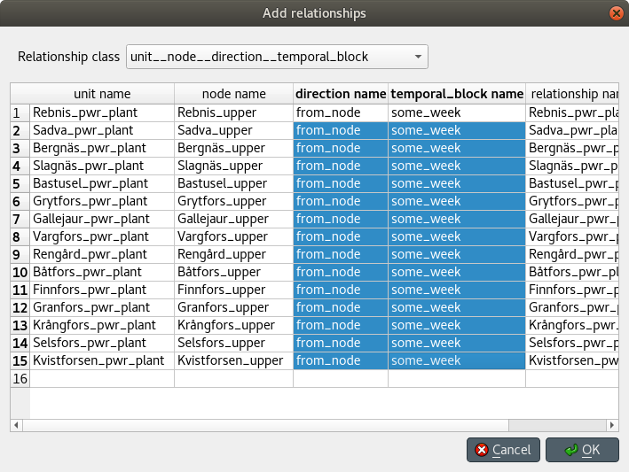

      

      Tip

      To enter the same text on several cells, copy the text into the clipboard, then select all target cells and press Ctrl+V.

   6. Click Ok.

   7. Back in the Data store tree view, under Relationship tree, double click on unit__node__direction__temporal_block to confirm that the relationships are effectively there.

   8. From the main menu, select Session -> Commit to open the Commit changes dialog. Enter “Add sending nodes of power plants” as the commit message and click Commit.

2. Repeat the procedure to establish that power plant units release water to the station’s lower node at each time slice in the one week horizon, as relationships of class unit__node__direction__temporal_block: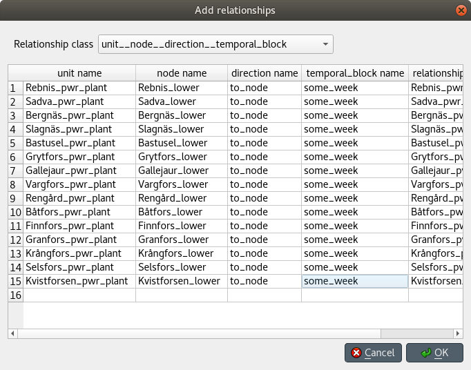

   

3. Repeat the procedure to establish that power plant units release electricity to the common electricity node at each time slice in the one week horizon, as relationships of class unit__node__direction__temporal_block:

   

4. Repeat the procedure to establish that reservoir units take and release water to and from the station’s upper node at each time slice in the one week horizon, as relationships of class unit__node__direction__temporal_block: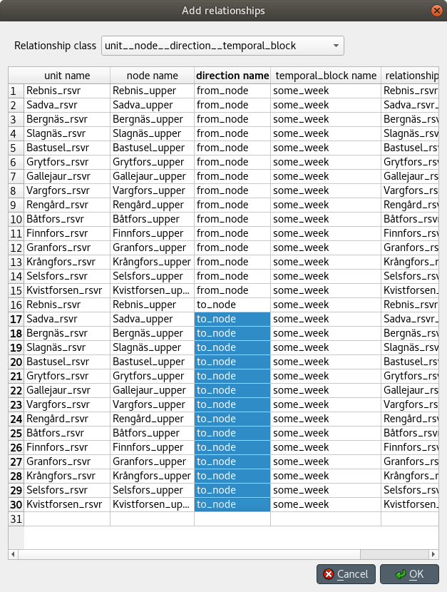

   

5. Repeat the procedure to establish that the electricity load takes electricity from the common electricity node at each time slice in the one week horizon, as a relationship of class unit__node__direction__temporal_block: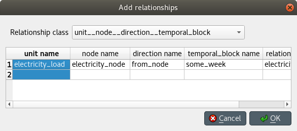

   

6. Repeat the procedure to establish that discharge connections take water from the lower node of one station and release it to the upper node of the downstream station, at each time slice in the one week horizon, as relationships of class connection__node__direction__temporal_block: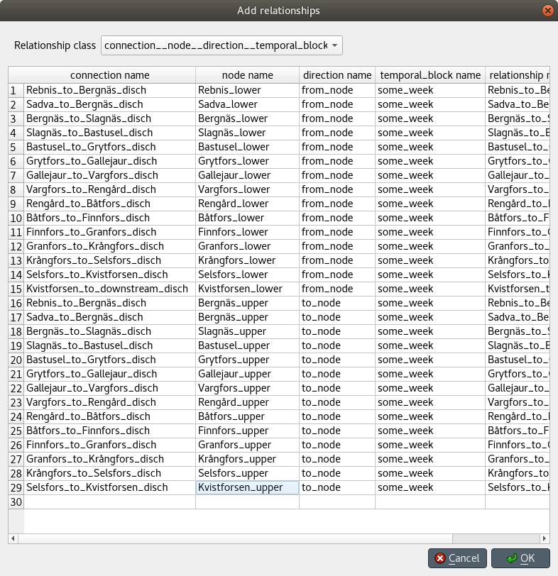

   

7. Repeat the procedure to establish that spillway connections take water from the upper node of one station and release it to the upper node of the downstream station, at each time slice in the one week horizon, as relationships of class connection__node__direction__temporal_block:

   

8. Repeat the procedure to establish that water nodes balance water, and the electricity node balances electricity, as relationships of class node__commodity: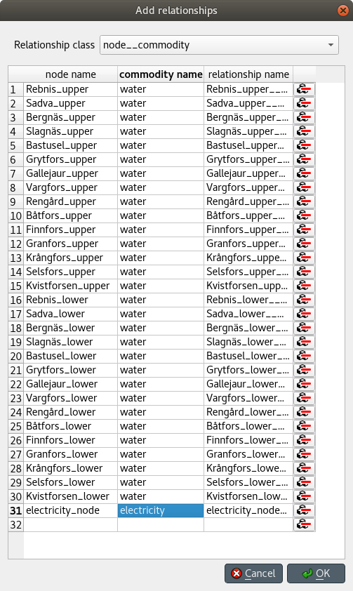

   

9. Repeat the procedure to establish that all nodes are balanced at each time slice in the one week horizon, as relationships of class node__temporal_block: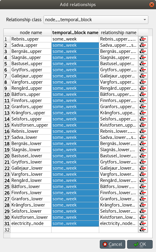

   

10. Repeat the procedure to establish the connection of each storage to the corresponding unit, as relationships of class storage__unit: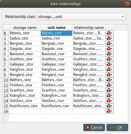

    

11. Repeat the procedure to establish that all storages store water, as relationships of class storage__commodity: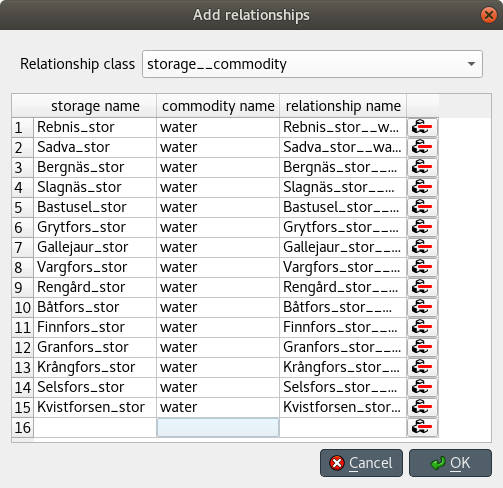

    

Specifying relationship parameter values

TODO

Running Spine model

Configuring Julia

1. Go to Spine Toolbox mainwindow and from the main menu, select File -> Settings. This will open the Settings dialog.
2. Go to the Julia group box and enter the path to your julia executable in the first line edit.
3. (Optional) Enter the path of a julia project that you want to use with Spine Toolbox in the second line edit. Leave blank to use julia’s home project.
4. Click Ok.
5. From the application main menu, select File -> Tool configuration assistant. This will install the Spine Model package to the julia project specified above. Follow the instructions until completion.

Creating a Tool template for Spine Model

TODO